AFNI Part 1: Introduction

As promised, we now begin our series of AFNI tutorials. These walkthroughs will be more in-depth than the FSL series, as I am more familiar with AFNI and use it for a greater number of tasks; accordingly, more advanced tools and concepts will be covered.

Using AFNI requires a solid understanding of Unix; the user should know how to write and read conditional statements and for loops, as well as know how to interpret scripts written by others. Furthermore, when confronted with a new or unfamiliar script or command, the user should be able to make an educated guess about what it does. AFNI also demands a sophisticated knowledge of fMRI preprocessing steps and statistical analysis, as AFNI allows the user more opportunity to customize his script.

A few other points about AFNI:

1) There is no release schedule. This means that there is no fixed date for the release of new versions or patches; rather, AFNI responds to user demands on an ad hoc basis. In a sense, all users are beta testers for life. The advantage is that requests are addressed quickly; I once made a feature request at an AFNI bootcamp, and the developers updated the software before I returned home the following week.

2) AFNI is almost entirely run from the command line. In order to make the process less painful, the developers have created "uber" scripts which allow the user to input experiment information through a graphical user interface and generate a preprocessing script. However, these should be treated as templates subject to further alteration.

3) AFNI has a quirky, strange, and, at times, shocking sense of humor. Through clicking on a random hotspot on the AFNI interface, one can choose their favorite Shakespeare sonnet; read through the Declaration of Independence; generate an inspirational quote or receive kind and thoughtful parting words. Do not let this deter you. As you become more proficient with AFNI, and as you gain greater life experience and maturity, the style of the software will become more comprehensible, even enjoyable. It is said that one knows he going insane when what used to be nonsensical gibberish starts to take on profound meaning. So too with AFNI.

The next video will cover the to3d command and the conversion of raw volumetric data into AFNI's BRIK/HEAD format; study this alongside data conversion through mricron, as both produce a similar result and can be used to complement each other. As we progress, we will methodically work through the preprocessing stream and how to visualize the output with AFNI, with an emphasis on detecting artifacts and understanding what is being done at each step. Along the way different AFNI tools and scripts will be broken down and discussed.

At long last my children, we shall take that which is rightfully ours. We shall become as gods among fMRI researchers - wise as serpents, harmless as doves. Seek to understand AFNI with an open heart, and I will gather you unto my terrible and innumerable flesh and hasten your annihilation.

FSL Tutorial 3: Running The Analysis

The end of our last set of tutorials covered the FEAT interface; and although there is much more there to explore and use, such as MELODIC's independent component analysis, for now we will simplify things and focus on a traditional, straightforward univariate analysis.

A few terms are worth defining here. First, whenever you read an instruction manual outlining how to set up and run a model with fMRI data, you will inevitably run into the term voxel-wise analysis. (Maybe not inevitably, but the point is, enough researchers and software packages use it to merit an acquaintance with it.) What this means is that we first construct a model of what we believe will happen at each voxel in the brain, given our timing files of what happened when. If, for example, ten seconds into the experiment the subject pressed a button with his right hand, we would expect to see a corresponding activation in the left motor cortex. When we talk about activation, we simply mean whether our model is a good fit or not for the signal observed in that voxel; and this model is generated by convolving - also known as the application of a moving average, a concept which is more easily explained through an animation found here - each event with a basis function, the most common and intuitive of which is a gamma function. Essentially what this boils down to is pattern matching in time; the better the fit for a particular contrast or condition, the more likely we are to believe that that particular voxel is responsive to that condition.

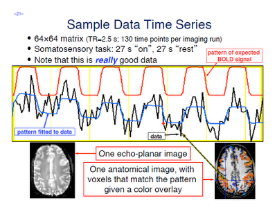
This image was stolen (literally) from the AFNI website educational material. Note that the red line is the ideal fit, while the blue line is the ideal fit scaled by a certain amount in order to fit the data. These scalars are also called beta weights; we will have "The Talk" about these at a later time, but only after you have reached fMRI maturity.

Furthermore, within the output of FEAT you will see plotted timecourses for each peak voxel for each contrast. The red line represents the raw signal timeseries at that voxel, which, as you can see, is relatively noisy, although it is clear when certain conditions were present. It should be noted that this experiment is a special case, as we are dealing with a block design which elicits robust activation in the left and right motor cortices; most studies employing event-related designs have much noisier data which is much more difficult to interpret. The blue line represents the complete model fit; that is, given all of the regressors, whether any activation in this voxel can be attributed to any of your conditions. Lastly, the green line represents only the contrast or condition of interest, and is usually only meaningful when looking at simple effects (i.e., undifferentiated contrasts which compare only one condition to the baseline signal present in the data).

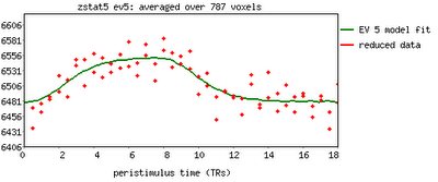
One feature not covered in this video tutorial is the visualization of peristimulus plots, which allow the user to see averages of the event over multiple repetitions. It provides much of the same information as the basic timeseries plots, but from a slightly different vantage point; you can see what timepoints are averaged, exactly, and how this contributes to the observed model fit.

Now that you have had FEAT guide you by the hand through your results, it is time to get down and dirty and look at your results in the output directories by yourself. FEAT generates a lot of output, but only a fraction of it is worth investigating for the beginning researcher, and almost all of it can be found in the stats directory. We will cover this in the following tutorial; for now, check your freezer for Hot Pockets.

FSL Tutorial 2: FEAT (Part 1)

A new tutorial about FEAT is now up; depending on how long it takes to get through all of the different tabs in the interface, this may be a three-part series. In any case, this will serve as a basic overview of the preprocessing steps of FEAT, most of which can be left as a default.

The next couple of tutorials will cover the set up of models and timing files within FSL, which can be a little tricky. For those of you who have stuck with it from the beginning (and I have heard that there are a few of you out there: Hello), there will be some more useful features coming up, aside from reviewing the basics.

Eventually we will get around to batch scripting FEAT analyses, which can save you several hours of mindless pointing and clicking, and leave you with plenty of time to watch Starcraft 2 replays, or Breaking Bad, or whatever it is kids watch these days.

FSL Tutorial: Part 1 (of many)

I recently started testing out FSL to see if it has any advantages over other fMRI analysis packages, and decided to document everything on Youtube as I go along. The concepts are the same as any other package (AFNI, SPM, etc), but the terminology is slightly different, and driving it from the command line is not as intuitive as you would think. Plus, they use a ton of acronyms for everything, which, to be honest, kind of pisses me off; I don't like it when they try to be cute and funny like that. The quotes and sonnets generated by AFNI after exiting the program, however, are sophisticated and endearing. One of my favorites: "Each goodbye makes the next hello closer!"

In any case, here is the first, introductory tutorial I made about FSL. I realized from searching around on Youtube that hardly any fMRI analysis tutorial videos exist, and that this is a market that sorely needs to be filled. A series of walkthroughs and online lessons using actual data, in my opinion, would be far more useful at illustrating the fundamentals of fMRI data analysis than only having manuals (although those are extremely important as well, and I would recommend that anyone getting started in the field read them so that they can needlessly suffer as I did).

I will attempt to upload more on a regular basis, and start to get some coherent lesson plan going which allows the beginner to get off the ground and understand what the hell is going on. True story: It took me at least three years to fully comprehend what a beta weight was. Three years. I'm not going to blame it all on Smirnoff Ice, but it certainly didn't help.

Note: I suggest hitting fullscreen mode and viewing at a higher resolution (360p or 480p) in order to better see the text in the terminal window.

Also, the example data for these tutorials can be found here.