Manually typing in contrasts in SPM is a grueling process that can have a wide array of unpleasant side effects, including diplopia, lumbago, carpal tunnel syndrome, psychosis, violent auditory and visual hallucinations, hives, and dry mouth. These symptoms are only compounded by the number of regressors in your model, and the number of subjects in your study.
Fortunately, there is a simply way to automate all of this - provided that each subject has the same number of runs, and that the regressors in each run are structured the same way. If they are, though, the following approach will work.
First, open up SPM and click on the TASKS button in the upper right corner of the Graphics window. The button is marked "TASKS" in capital letters, because they really, really want you to use this thing, and mitigate all of the damage and harm in your life caused by doing things manually. You then select the Stats menu, then Contrast Manager. The options from there are straightforward, similar to what you would do when opening up the Results section from the GUI and typing in contrasts manually.
When specifying the contrast vector, take note of how many runs there are per subject. This is because we want to take the average parameter estimate for each regressor we are considering; one can imagine a scenario where one of the regressors occurs in every run, but the other regressor only happens in a subset of runs, and this more or less puts them on equal footing. In addition, comparing the average parameter or contrast estimate across subjects is easier to interpret.
Once you have the settings to your satisfaction, save it out as a .mat file - for example, 'RunContrasts.mat'. This can then be loaded from the command line:
load('RunContrasts')
Which will put a structure called "jobs" in your workspace, which contains all of the code needed to run a first-level contrast. The only part of it we need to change when looping over subjects is the spmmat field, which can be done with code like the following:
subjList=[207 208]; %And so on, including however many subjects you want
for subj=subjList
jobs{1}.stats{1}.con.spmmat = {['/data/hammer/space4/MultiOutcome2/fmri/' num2str(subj) '/RESULTS/model_multiSess/SPM.mat']} %This could be modified so that the path is a variable reflecting where you put your SPM.mat file
spm_jobman('run', jobs)
end
This is demonstrated in the following pair of videos; the first, showing the general setup, and the second showing the execution from the command line.


