Central Limit Theorem Part 2: Retaliation

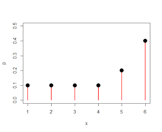
Discrete population, with different probabilities associated with different numbers

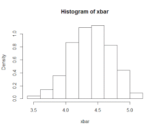
Sampling distribution of means from the discrete parent population, with a sample size of n=30

In the last post, we left the central limit theorem defined as a normally-distributed sampling distribution of means reflecting the shape of the normally-distributed parent population, but with a smaller spread and less variance. However, what happens when we sample from a non-normal distribution, such as an exponential distribution or a discrete distribution?

As it turns out, the sampling distribution of means is also normal, regardless of the shape of the parent population. This holds for sample sizes of about 30 or more, which is why the central limit theorem is also sometimes referred to as the law of large numbers.

This is shown in the following video, and can be modified with this R script.

The Central Limit Theorem: Part 1

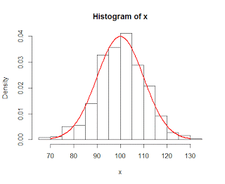
Random sample of numbers from a normal distribution, N ~ (100, 10). Actual normal distribution is superimposed in red.

One fundamental concept for hypothesis testing is something called the Central Limit Theorem. This theorem states that, for large enough sample sizes and for enough samples, we begin to build a sampling distribution that is approximately normal. More importantly, when we build sampling distributions of the means selected from a population, the average mean is identical to the mean of the parent population.

To illustrate this in R, from the parent population we can take random samples of several different sizes - 10, 50, 300 - and plot those samples as a histogram. These samples will roughly follow the shape of the population they were drawn from - in this case, the normal distribution with a mean of 100 and a standard deviation of 10 - and the more observations we have in our sample, the more closely it reflects the actual parent population. Theoretically, if our sample were large enough, it would in essence sample the entire population and therefore be the same as the population.

However, for smaller sample sizes, we can calculate the mean of each sample and then plot that value in a histogram. If we do this enough times, the mean of the sampling distribution has less spread and more tightly clusters around the mean of the parent population. Increasing the sample size does the same thing.

The demo script can be downloaded here; I have basically copied the code from this website, but distilled it into an R script that can be used and modified by anybody.