Introduction to Reinforcement Learning Models

Someone very near and dear to me just sent me a picture of herself cuddled up on the couch in her pajamas with an Argentinian Tegu. That's right lady, I said Tegu. The second coming of Sodom and Gomorrah - you heard it here first, folks! I mean, I know it's the twenty-first century and all, but what the heck.

Looks like I'll be pushing her to buy that lucrative life insurance policy much earlier than planned!

Anyway, I think that little paroxysm of righteous anger provides an appropriate transition into our discussion of reinforcement learning. Previously we talked about how a simple model can simulate an organism processing a stimulus, such as a tone, and begin to associate that with rewards or lack of rewards, which in turn leads to either greater levels of dopamine firing, or depressed levels of dopamine firing. Over time, dopamine firing begins to respond to the conditioned stimulus itself instead of the reward as it becomes more tightly linked to receiving the reward in the near future. This phenomenon is so strong and reliable across all species, it can even be observed in the humble sea slug Aplysia, which is one ugly sucker if I've ever seen one. Probably wouldn't stop her from cuddling up with that monstrosity, though!

Anyway, that only describes one form of learning - to wit, classical conditioning. (Do you think I am putting on airs when I use a phrase like "to wit"? She thinks that I do; but then again, she also has passionate, perverted predilections for cold-blooded wildlife.) Obviously, any animal in the food chain - even the ones she associates with - can be classically conditioned to almost anything. Much more interesting is operant conditioning, in which an individual has to make certain choices, or actions, and then evaluate the consequences of those choices. Kind of like hugging reptiles! Oh hey, she probably thinks, let's see if hugging this lizard - this pebbly-skinned, fork-tongued, unblinking beast - results in some kind of reward, like gold coins shooting out of my mouth. In operant conditioning parlance, the rush of gold coins flowing out of one's orifice would be a reinforcer, which increases the probability of that action in the future; while a negative event, such as being fatally bitten by the reptile - which pretty much any sane person would expect to happen - would be a punisher, which decreases the probability of that action in the future.

The classically conditioned responses, in other words, serve the function of a critic which monitors for stimuli and reliably-predicted reinforcers or punishers following those stimuli, while operant conditioning can be thought of as an actor role, where choices are made and the results evaluated against what was expected. Sutton and Barto, a pair of researchers considerably less sanguinary than Hodgkin and Huxley, were among the first to propose and refine this model, assigning the critic role to the ventral striatum and the actor role to the dorsal striatum. So, that's where they are; if you want to find the actor component of reinforcement learning, for example, just grab a flashlight and examine the dorsal striatum inside someone's skull, and, hey presto! there it is. I won't tell you what it looks like.

However, we can form some abstract idea about what the actor component looks like by simulating it in Matlab. No, just in case you were wondering, this won't help you hook up with Komodo Dragons! It will, however, refine our understanding of how reinforcement learning works, by building upon the classical conditioning architecture we discussed previously. In this case, weights are still updated, but now we have two actions to choose from, which results in four combinations: either one or the other, both at the same time, or neither. In this example, only doing action 1 will lead to a reward, and this gets learned right quick by the simulation. As before, a surface map of delta shows the reward signal being transferred from the actual reward itself to the action associated with that reward, and a plot of the vectors shows action 1 clearly dominating over action 2. The following code will help you visualize these plots, and see how tweaking parameters such as the discount factor and learning rate affect delta and the action weights. But it won't help you get those gold coins, will it?


clear
clc
close all

numTrials = 200;
numSteps = 100;
weights = zeros(100,200); %Array of weights from steps 1-100, initialized to zero

discFactor = 0.995; %Discounting factor
learnRate = 0.3; %Learning Rate
delta = zeros(100,200); %Empty vector
V = []; %Empty vector
x = [zeros(1,19) ones(1,81)];

r = zeros(100,200); %Reward vector, which will be populated with 1's whenever a reward occurs (in this case, when action1 == 1 and action2 == 0)

W1=0;
W2=0;
a1=zeros(1,numTrials);
a2=zeros(1,numTrials);


for idx = 1:numTrials
   
    for t = 1:numSteps-1
        if t==20
            as1=x(t)*W1; %Compute action signals at time step 20 within each trial
            as2=x(t)*W2;
           
            ap1 =  exp(as1)/(exp(as1)+exp(as2)); %Softmax function to calculate probability associated with each action
            ap2 =  exp(as2)/(exp(as1)+exp(as2));
           
            n=rand;
            if n<(idx)=1;
            end
           
            n=rand;
            if n<ap2                a2(idx)=1;
            end
        
            if a1(idx)==1 && a2(idx)==0 %Only deliver reward when action1 ==1 and action2 ==0
                r(50:55,idx)=1;
            end                       
        end
       
        V(t,idx) = x(t).*weights(t, idx);
        V(t+1,idx) = x(t+1).*weights(t+1, idx);
       
        delta(t+1,idx) = r(t+1,idx) + discFactor.*V(t+1,idx) - V(t,idx);
       
        weights(t, idx+1) = weights(t, idx)+learnRate.*x(t).*delta(t+1,idx);
       
        W1 = W1 + learnRate*delta(t+1,idx)*a1(idx);
        W2 = W2 + learnRate*delta(t+1,idx)*a2(idx);
       
    end
   
    w1Vect(idx) = W1;
    w2Vect(idx) = W2;


end


figure
set(gcf, 'renderer', 'zbuffer') %Can prevent crashes associated with surf command
surf(delta)

figure
hold on
plot(w1Vect)
plot(w2Vect, 'r')


======================

Oh, and one more thing that gets my running tights in a twist - people who don't like Bach. Who the Heiligenstadt Testament doesn't like Bach? Philistines, pederasts, and pompous, nattering, Miley Cyrus-cunnilating nitwits, that's who! I get the impression that most people have this image of Bach as some bewigged fogey dithering around in a musty church somewhere improvising fugues on an organ, when in fact he wrote some of the most hot-blooded, sphincter-tightening, spiritually liberating music ever composed. He was also, clearly, one of the godfathers of modern metal; listen, for example, to the guitar riffs starting at 6:38.


...Now excuse me while I clean up some of the coins off the floor...

Introduction to Computational Modeling: Hodgkin-Huxley Model

Computational modeling can be a tough nut to crack. I'm not just talking pistachio-shell dense; I'm talking walnut-shell dense. I'm talking a nut so tough that not even a nutcracker who's cracked nearly every damn nut on the planet could crack this mother, even if this nutcracker is so badass that he wears a leather jacket, and that leather jacket owns a leather jacket, and that leather jacket smokes meth.

That being said, the best approach to eat this whale is with small bites. That way, you can digest the blubber over a period of several weeks before you reach the waxy, delicious ambergris and eventually the meaty whale guts of computational modeling and feel your consciousness expand a thousandfold. And the best way to begin is with a single neuron.


The Hodgkin-Huxley Model, and the Hunt for the Giant Squid

Way back in the 1950s - all the way back in the twentieth century - a team of notorious outlaws named Hodgkin and Huxley became obsessed and tormented by fevered dreams and hallucinations of the Giant Squid Neuron. (The neurons of a giant squid are, compared to every other creature on the planet, giant. That is why it is called the giant squid. Pay attention.)

After a series of appeals to Holy Roman Emperor Charles V and Pope Stephen II, Hodgkin and Huxley finally secured a commission to hunt the elusive giant squid and sailed to the middle of the Pacific Ocean in a skiff made out of the bones and fingernails and flayed skins of their enemies. Finally spotting the vast abhorrence of the giant squid, Hodgkin and Huxley gave chase over the fiercest seas and most violent winds of the Pacific, and after a tense, exhausting three-day hunt, finally cornered the giant squid in the darkest netherregions of the Marianas Trench. The giant squid sued for mercy, citing precedents and torts of bygone eras, quoting Blackstone and Coke, Anaxamander and Thales. But Huxley, his eyes shining with the cold light of purest hate, smashed his fist through the forehead of the dread beast which erupted in a bloody Vesuvius of brains and bits of bone both sphenoidal and ethmoidal intermixed and Hodgkin screamed and vomited simultaneously. And there stood Huxley triumphant, withdrawing his hand oversized with coagulate gore and clutching the prized Giant Squid Neuron. Hodgkin looked at him.

"Huxley, m'boy, that was cold-blooded!" he ejaculated.
"Yea, oy'm one mean cat, ain't I, guv?" said Huxley.
"'Dis here Pope Stephen II wanted this bloke alive, you twit!"
"Oy, not m'fault, guv," said Huxley, his grim smile twisting into a wicked sneer. "Things got outta hand."


Scene II

Drunk with victory, Hodgkin and Huxley took the Giant Squid Neuron back to their magical laboratory in the Ice Cream Forest and started sticking a bunch of wires and electrodes in it. To their surprise, there was a difference in voltage between the inside of the neuron and the bath surrounding it, suggesting that there were different quantities of electrical charge on both sides of the cell membrane. In fact, at a resting state the neuron appeared to stabilize around -70mV, suggesting that there was more of a negative electrical charge inside the membrane than outside.

Keep in mind that when our friends Hodgkin and Huxley began their quest, nobody knew exactly how the membrane of a neuron worked. Scientists had observed action potentials and understood that electrical forces were involved somehow, but until the experiments of the 1940s and '50s the exact mechanisms were still unknown. However, through a series of carefully controlled studies, the experimenters were able to measure how both current and voltage interacted in their model neuron. It turned out that three ions - sodium (Na+), potassium (K+), and chlorine (Cl-) - appeared to play the most important role in depolarizing the cell membrane and generating an action potential. Different concentrations of the ions, along with the negative charge inside the membrane, led to different pressures exerted on each of the ions.

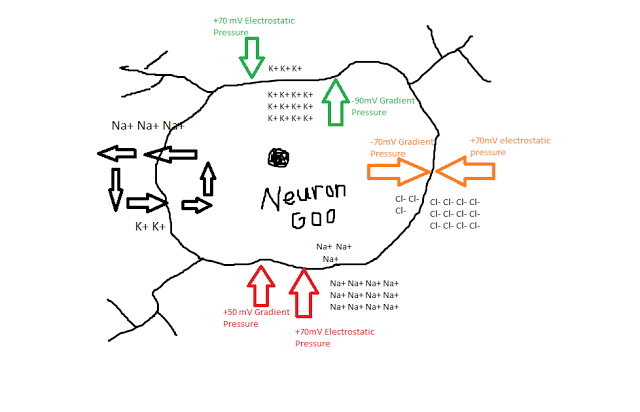
For example, K+ was found to be much more concentrated inside of the neuron than outside, leading to a concentration gradient exerting pressure for the K+ ions to exit the cell; at the same time, however, the attractive negative force inside the membrane exerting a countering electrostatic pressure, as positively charged potassium ions would be drawn toward the inside of the cell. Similar characteristics of the sodium and chlorine ions were observed as well, as shown in the following figure:

Ned the Neuron, filled with Neuron Goo. Note that the gradient and electrostatic pressures, expressed in microvolts (mV) have arbitrary signs; the point is to show that for an ion like chlorine, the pressures cancel out, while for an ion like potassium, there is slightly more pressure to exit the cell than enter it. Also, if you noticed that these values aren't 100% accurate, then congratu-frickin-lations, you're smarter than I am, but there is no way in HECK that I am redoing this in Microsoft Paint.


In addition to these passive forces, Hodgkin and Huxley also observed an active, energy-consuming force in maintaining the resting potential - a mechanism which exchanged potassium for sodium ions, by kicking out roughly three sodium ions for each potassium ion. Even with this pump though, there is still a whopping 120mV of pressure for sodium ions to enter. What prevents them from rushing in there and trashing the place?

Hodgkin and Huxley hypothesized that certain channels in the neuron membrane were selectively permeable, meaning that only specific ions could pass through them. Furthermore, channels could be either open or closed; for example, there may be sodium channels dotting the membrane, but at a resting potential they are usually closed. In addition, Hodgkin and Huxley thought that within these channels were gates that regulated whether the channel was open or closed, and that these gates could be in either permissive or non-permissive states. The probability of a gate being in either state was dependent on the voltage difference between the inside and the outside of the membrane.

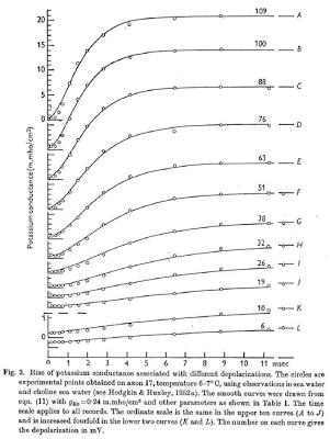
Although this all may seem conceptually straightforward, keep in mind that Hodgkin and Huxley were among the first to combine all of these properties into one unified model - something which could account for the conductances, voltage, and current, as well as how all of this affected the gates within each ion channel - and they were basically doing it from scratch. Also keep in mind that these crazy mofos didn't have stuff like Matlab or R to help them out; they did this the old-fashioned way, by changing one thing at a time and measuring that shit by hand. Insane. (Also think about how, in the good old days, people like Carthaginians and Romans and Greeks would march across entire continents for months, years sometimes, just to slaughter each other. Continents! These days, my idea of a taxing cardiovascular workout is operating a stapler.) To show how they did this for quantifying the relationship between voltage and conductance in potassium, for example, they simply applied a bunch of different currents, saw how it changed over time, and attempted to fit a mathematical function to it, which happens to fit quite nicely when you include n-gates and a fourth-power polynomial.


After a series of painstaking experiments and measurements, Hodgkin and Huxley calculated values for the conductances and equilibrium voltages for different ions. Quite a feat, when you couple that with the fact that they hunted down and killed their very own Giant Squid and then ripped a neuron out of its brain. Incredible. That is the very definition of alpha male behavior, and it's something I want all of my readers to emulate.
Table 3 from Hodgkin & Huxley (1952) showing empirical values for voltages and conductances, as well as the capacitance of the membrane.

The same procedure was used for the n, m, and h gates, which were also found to be functions of the membrane voltage. Once these were calculated, then the conductances and voltage potential could be found for any resting potential and any amount of injected current.

H & H's formulas for the n, m, and h gates as a function of voltage.

So where does that leave us? Since Hodgkin and Huxley have already done most of the heavy lifting for us, all we need to do is take their constants and equations they've already derived, and put it into a script that we can then run through Matlab. At some point, just to get some additional exercise, we may also operate a stapler.

But stay focused here. Most of the formulas and constants can simply be transcribed from their papers into a Matlab script, but we also need to think about the final output that we want, and how we are going to plot it. Note that the original Hodgkin and Huxley paper uses a differential formula for voltage to tie together the capacitance and conductance of the membrance, e.g.:

We can use a method like Euler first-order approximation to plot the voltages, in which each time step is based off of the previous one which is added to a function multiplied by a time step; in the sample code below, the time step can be extremely small, thus giving a better approximation to the true shape of the voltage timecourse. (See the "calculate the derivatives" section below.)

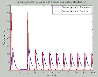
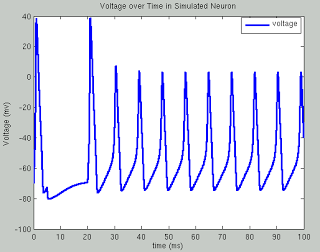
The following code runs a simulation of the Hodgkin Huxley model over 100 milliseconds with 50mA of current, although you are encouraged to try your own and see what happens. The sample plots below show the results of a typical simulation; namely, that the voltage depolarizes after receiving a large enough current and briefly becomes positive before returning to its previous resting potential. The conductances of sodium and potassium show that the sodium channels are quickly opened and quickly closed, while the potassium channels take relatively longer to open and longer to close.The point of the script is to show how equations from papers can be transcribed into code and then run to simulate what neural activity should look like under certain conditions. This can then be expanded into more complex areas such as memory, cognition, and learning.

The actual neuron, of course, is nowhere to be seen; and thank God for that, else we would run out of Giant Squids before you could say Jack Robinson.


Resources
Book of GENESIS, Chapter 4
Original Hodgkin & Huxley paper


%===simulation time===
simulationTime = 100; %in milliseconds
deltaT=.01;
t=0:deltaT:simulationTime;


%===specify the external current I===
changeTimes = [0]; %in milliseconds
currentLevels = [50]; %Change this to see effect of different currents on voltage (Suggested values: 3, 20, 50, 1000)

%Set externally applied current across time
%Here, first 500 timesteps are at current of 50, next 1500 timesteps at
%current of zero (resets resting potential of neuron), and the rest of
%timesteps are at constant current
I(1:500) = currentLevels; I(501:2000) = 0; I(2001:numel(t)) = currentLevels;
%Comment out the above line and uncomment the line below for constant current, and observe effects on voltage timecourse
%I(1:numel(t)) = currentLevels;


%===constant parameters===%
%All of these can be found in Table 3
gbar_K=36; gbar_Na=120; g_L=.3;
E_K = -12; E_Na=115; E_L=10.6;
C=1;


%===set the initial states===%
V=0; %Baseline voltage
alpha_n = .01 * ( (10-V) / (exp((10-V)/10)-1) ); %Equation 12
beta_n = .125*exp(-V/80); %Equation 13
alpha_m = .1*( (25-V) / (exp((25-V)/10)-1) ); %Equation 20
beta_m = 4*exp(-V/18); %Equation 21
alpha_h = .07*exp(-V/20); %Equation 23
beta_h = 1/(exp((30-V)/10)+1); %Equation 24

n(1) = alpha_n/(alpha_n+beta_n); %Equation 9
m(1) = alpha_m/(alpha_m+beta_m); %Equation 18
h(1) = alpha_h/(alpha_h+beta_h); %Equation 18


for i=1:numel(t)-1 %Compute coefficients, currents, and derivates at each time step
   
    %---calculate the coefficients---%
    %Equations here are same as above, just calculating at each time step
    alpha_n(i) = .01 * ( (10-V(i)) / (exp((10-V(i))/10)-1) );
    beta_n(i) = .125*exp(-V(i)/80);
    alpha_m(i) = .1*( (25-V(i)) / (exp((25-V(i))/10)-1) );
    beta_m(i) = 4*exp(-V(i)/18);
    alpha_h(i) = .07*exp(-V(i)/20);
    beta_h(i) = 1/(exp((30-V(i))/10)+1);
   
   
    %---calculate the currents---%
    I_Na = (m(i)^3) * gbar_Na * h(i) * (V(i)-E_Na); %Equations 3 and 14
    I_K = (n(i)^4) * gbar_K * (V(i)-E_K); %Equations 4 and 6
    I_L = g_L *(V(i)-E_L); %Equation 5
    I_ion = I(i) - I_K - I_Na - I_L;
   
   
    %---calculate the derivatives using Euler first order approximation---%
    V(i+1) = V(i) + deltaT*I_ion/C;
    n(i+1) = n(i) + deltaT*(alpha_n(i) *(1-n(i)) - beta_n(i) * n(i)); %Equation 7
    m(i+1) = m(i) + deltaT*(alpha_m(i) *(1-m(i)) - beta_m(i) * m(i)); %Equation 15
    h(i+1) = h(i) + deltaT*(alpha_h(i) *(1-h(i)) - beta_h(i) * h(i)); %Equation 16

end


V = V-70; %Set resting potential to -70mv

%===plot Voltage===%
plot(t,V,'LineWidth',3)
hold on
legend({'voltage'})
ylabel('Voltage (mv)')
xlabel('time (ms)')
title('Voltage over Time in Simulated Neuron')


%===plot Conductance===%
figure
p1 = plot(t,gbar_K*n.^4,'LineWidth',2);
hold on
p2 = plot(t,gbar_Na*(m.^3).*h,'r','LineWidth',2);
legend([p1, p2], 'Conductance for Potassium', 'Conductance for Sodium')
ylabel('Conductance')
xlabel('time (ms)')
title('Conductance for Potassium and Sodium Ions in Simulated Neuron')


Comprehensive Computational Model of ACC: Expected Value of Control

Figure 1: Example of cognitive control failure

A new comprehensive computational model of dorsal anterior cingulate cortex function (dACC) was published in last week's issue of Neuron, sending shockwaves throughout the computational modeling community and sending computational modelers running to neuroscience magazinestands in droves. (That's right, I used the word droves - and you know I reserve that word only for special cases.)

The new model, published by Shenhav, Botvinick, and Cohen, attempts to unify existing models and empirical data of dACC function by modifying the traditional monitoring role usually ascribed to the dACC. In previous models of dACC function, such as error detection and conflict monitoring, the primary role of the dACC was that of a monitor involved in detecting errors, or monitoring for mutually exclusive responses and signaling the need to override prepotent but potentially wrong responses. The current model, on the other hand, suggests that the dACC monitors the expected value associated with certain responses, and weighs the potential cost of recruiting more cognitive control against the potential value (e.g., reward or other positive outcome) for implementing cognitive control.

This kind of tradeoff is best illustrated with a basic task like the Stroop task, where a color word - such as "green" - is presented in an incongruent ink, such as red. The instructions in this task are to respond to the color, and not the word; however, this is difficult since reading a word is an automatic process. Overriding this automatic tendency to respond to the word itself requires cognitive control, or strengthening task-relevant associations - in this case, focusing more on the color and not the word itself.

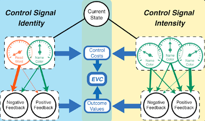
However, there is a drawback: using cognitive control requires effort, and effort isn't always pleasant. Therefore, it stands to reason that the positives for expending this mental effort should outweigh the negatives of using cognitive control. The following figure shows this as a series of meters with greater cognitive control going from left to right:

Figure 1B from Shenhav et al, 2013
As the meters for control signal intensity increase, so does the probability of choosing the correct option that will lead to positive feedback, as shown by the increasing thickness of the arrows from left to right. The role of the dACC, according to the model, is to make sure that the amount of cognitive control implemented is optimal: if someone always goes balls-to-the-wall with the amount of cognitive control they bring to the table, they will probably expend far more energy then would be necessary, even though they would have a much higher probability of being correct every time. (Study question: Do you know anybody like this?) Thus, the dACC attempts to reach a balance between the cognitive control needed and the value of the outcome, as shown in the middle column of the above figure.

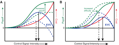
This balance is referred to as the expected value of control (EVC): the difference between control costs and outcome values you can expect for a range of control signal intensities. The expected value can be plotted as a curve integrating both the costs and benefits of increased control, with a clear peak at the level of intensity that maximizes the difference between the expected payoff and control cost (Figure 2):

EVC curves (in blue) integrating costs and payoffs for control intensity. (Reproduced from Figure 4 from Shenhav et al, 2013)

That, in very broad strokes, is the essence of the EVC model. There are, of course, other aspects to it, including a role for the dACC in choosing the control identity which orients toward the appropriate behavior and response-outcome associations (for example, actually paying attention to the color of the stroop stimulus in the first place), which can be read about in further detail in the paper. Overall, the model seems to strike a good balance between complexity and conciseness, and the equations are relatively straightforward and should be easy to implement for anyone looking to run their own simulations.

So, the next time you see a supermodel in a bathtub full of Nutella inviting you to join her, be aware that there are several different, conflicting impulses being processed in your dorsal anterior cingulate. To wit, 1) How did this chick get in my bathtub? 2) How did she fill it up with Nutella? Do they sell that stuff wholesale at CostCo or something? and 3) What is the tradeoff between exerting enough control to just say no, given that eating that much chocolate hazelnut spread will cause me to be unable to move for the next three days, and giving in to temptation? It is a question that speaks directly to the human condition; between abjuring gluttony and the million ailments that follow on vice, and simply giving in, dragging that broad out of your bathtub and toweling the chocolate off her so you don't waste any of it, showing her the door, and then returning to the tub and plunging your insatiable maw into that chocolatey reservoir of bliss, that muddy fountain of pleasure, and inhaling pure ecstasy.

Computational Modeling: A Confession

File:fig cortical cons ff fb lat.png


In a desperate attempt to make myself look cool and connected, on my lab webpage I wrote that my research
...focuses on the application of fMRI and computational modeling in order to further understand prediction and evaluation mechanisms in the medial prefrontal cortex and associated cortical and subcortical areas...
Lies. By God, lies. I know as much about computational modeling as I do about how Band-Aids work or what is up an elephant's trunk. I had hoped that I would grow into the description I wrote for myself; but alas, as with my pathetic attempts to wake up every morning before ten o'clock, or my resolution to eat vegetables at least once a week, this also has proved too ambitious a goal; and slowly, steadily, I find myself engulfed in a blackened pit of despair.

Computational modeling - mystery of mysteries. In my academic youth I observed how cognitive neuroscientists outlined computational models of how certain parts of the brain work; I took notice that their work was received with plaudits and the feverish adoration of my fellow nerds; I then burned with jealousy upon seeing these modelers at conferences, mobs of slack-jawed science junkies surrounding their posters, trains of odalisques in their wake as they made their way back to their hotel chambers at the local Motel 6 and then proceeded to sink into the ocean of their own lust. For me, learning the secrets of this dark art meant unlocking the mysteries of the universe; I was convinced it would expand my consciousness a thousandfold.

I work with a computational modeler in my lab - he is the paragon of happiness. He goes about his work with zest and vigor, modeling anything and everything with confidence; not for a moment does self-doubt cast its shadow upon his soul. He is the envy of the entire psychology department; he has a spring in his step and a knowing wink in his eye; the very mention of his name is enough to make the ladies' heads turn. He has it all, because he knows the secrets, the joys, the unbounded ecstasies of computational modeling.

Desiring to have this knowledge for myself, I enrolled in a class about computational modeling. I hoped to gain some insight; some clarity. So far I have only found myself entangled in a confused mess. I hold onto the hope that through perseverance something will eventually stick.

However, the class has provided useful resources to get the beginner started. A working knowledge of the electrochemical properties of neurons is essential, as is modeling their effects through software such as Matlab. The Book of Genesis is a good place to get started with sample code and to catch up on the modeling argot; likewise, the CCN wiki over at Colorado is a well-written introduction to the concepts of modeling and how it applies to different cognitive domains.

I hope that you get more out of them than I have so far; I will post more about my journey as the semester goes on.