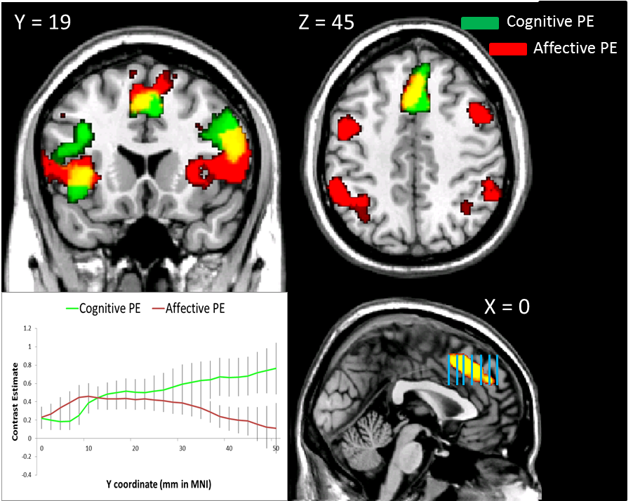
Slice analysis is a simple procedure - first you take a jar of peanut butter and a jar of Nutella, and then use a spoon to take some Nutella and then use the same spoon to mix it with the peanut butter. Eat and repeat until you go into insulin shock, and then...
No, wait! I was describing my midnight snack. The actual slice analysis method, although less delicious, is infinitely more helpful in determining regional dissociations of activity, as well as avoiding diabetes. (Although who says they can't both be done at the same time?)
The first step is to extract contrast estimates for each slice from a region of interest (ROI, also pronounced "ROY") and then average across all the voxels in that slice for the subject. Of course, there is no way you would be able to do this step on your own, so we need to copy someone else's code from the Internet and adapt it to our needs; one of John Ashburner's code snippets (#23, found here) is a good template to start with. Here is my adaptation:
rootdir = '/data/drill/space10/PainStudy/fmri/'; %Change these to reflect your directory structure
glmdir = '/RESULTS/model_RTreg/'; %Path to SPM.mat and mask files
subjects = [202:209 211:215 217 219 220:222 224:227 229 230 232 233];
%subjects = 202:203;
Conditions.names = {'stroopSurpriseConStats', 'painSurpriseConStats'}; %Replace with your own conditions
Masks = {'stroopSurpriseMask.img', 'painSurpriseMask.img'}; %Replace with your own masks; should be the product of a binary ROI multiplied by your contrast of interest
Conditions.Contrasts = {'', ''};
ConStats = [];
Condition1 = [];
Condition2 = [];
for i=subjects
cd([rootdir num2str(i) glmdir])
outputPath = [rootdir num2str(i) glmdir]; %Should contain both SPM.mat file and mask files
for maskIdx = 1:length(Masks)
P = [outputPath Masks{(maskIdx)}];
V=spm_vol(P);
tmp2 = [];
[x,y,z] = ndgrid(1:V.dim(1),1:V.dim(2),0);
for i=1:V.dim(3),
z = z + 1;
tmp = spm_sample_vol(V,x,y,z,0);
msk = find(tmp~=0 & isfinite(tmp));
if ~isempty(msk),
tmp = tmp(msk);
xyz1=[x(msk)'; y(msk)'; z(msk)'; ones(1,length(msk))];
xyzt=V.mat(1:3,:)*xyz1;
for j=1:length(tmp),
tmp2 = [tmp2; xyzt(1,j), xyzt(2,j), xyzt(3,j), tmp(j)];
end;
end;
end;
xyzStats = sortrows(tmp2,2); %Sort relative to second column (Y column); 1 = X, 3 = Z
minY = min(xyzStats(:,2));
maxY = max(xyzStats(:,2));
ConStats = [];
for idx = minY:2:maxY
x = find(xyzStats(:,2)==idx); %Go in increments of 2, since most images are warped to this dimension; however, change if resolution is different
ConStats = [ConStats; mean(xyzStats(min(x):max(x),4))];
end
if maskIdx == 1
Condition1 = [ConStats Condition1];
elseif maskIdx == 2
Condition2 = [ConStats Condition2];
end
end
end
Conditions.Contrasts{1} = Condition1;
Conditions.Contrasts{2} = Condition2;
This script assumes that there are only two conditions; more can be added, but care should be taken to reflect this, especially with the if/else statement near the end of the script. I could refine it to work with any amount of conditions, but that would require effort and talent.
Once these contrasts are loaded into your structure, you can then put them in an Excel spreadsheet or any other program that will allow you to format and save the contrasts in a tab-delimited text format. The goal is to prepare them for analysis in R, where you can test for main effects and interactions across the ROI for your contrasts. In Excel, I like to format it in the following four-column format:
Subject Condition Position Contrast
202 Stroop 0 -0.791985669
202 Stroop 2 -0.558366941
202 Stroop 4 -0.338829942
202 Pain 0 0.17158524
202 Pain 2 0.267789503
202 Pain 4 0.192473782
203 Stroop 0 0.596162455
203 Stroop 2 0.44917655
203 Stroop 4 0.410870348
203 Pain 0 0.722974284
203 Pain 2 0.871030304
203 Pain 4 1.045700207
And so on, depending on how many subjects, conditions, and slices you have. (Note here that I have position in millimeters from the origin in the y-direction; this will depend on your standardized space resolution, which in this case is 2mm per slice.)
Once you export that to a tab-delimited text file, you can then read it into R and analyze it with code like the following:
setwd("~/Desktop")
x = read.table("SliceAnalysis.txt", header=TRUE)
x$Subject <- as.factor="" font="" ubject="" x="">
aov.x = aov(Contrast~(Condition*Position)+Error(Subject/(Condition*Position)),x)
summary(aov.x)
interaction.plot(x$Position, x$Condition, x$Contrast)
This will output statistics for main effects and interactions, as well as plotting the contrasts against each other as a function of position.
That's it! Enjoy your slices, crack open some jars of sugary products, and have some wild times!

